Survival analysis

library(pipeML)
library(dplyr)
#> 
#> Attaching package: 'dplyr'
#> The following objects are masked from 'package:stats':
#> 
#>     filter, lag
#> The following objects are masked from 'package:base':
#> 
#>     intersect, setdiff, setequal, union

Survival outcomes

pipeML also trains models that predict time-to-event outcomes. The outcome has two components:

• time: follow-up or survival time
• event: whether the event occurred (1) or the observation was censored (0). It must be coded with these two values, without missing values.

Survival models are built with parsnip and its censored extension. censored must be installed, but you don’t need to load it: pipeML loads it when a survival task runs.

install.packages("censored")  # only needed once

Data

data_example_survival is the lung cancer dataset of the survival package: survival time in days, event indicator status (1 = death, 0 = censored) and 8 covariates.

data <- pipeML::data_example_survival
X <- data %>% dplyr::select(-time, -status)
time <- data$time
event <- data$status

Split the samples into a training and a test set, stratified by event:

set.seed(123)
train_idx <- caret::createDataPartition(event, p = 0.7, list = FALSE)

X_train <- X[train_idx, ]
X_test  <- X[-train_idx, ]
time_train <- time[train_idx]
time_test  <- time[-train_idx]
event_train <- event[train_idx]
event_test  <- event[-train_idx]

Train models

With task_type = "survival", compute_features.training.ML() trains and tunes six survival models (Cox proportional hazards, elastic-net Cox, parametric accelerated failure time model, conditional inference tree, bagged CART and oblique random survival forest) with repeated k-fold cross-validation stratified by event. time_var and event_var are the time and event of each training sample. The best model is selected by the concordance index (C-index).

As for classification, near-constant and highly correlated features (|r| > 0.9) are removed from the training features before the cross-validation (preprocess = TRUE, the default); none of the features of this example is removed.

Survival models are slower to train than classification models: here we use 3 folds and 1 repetition to keep the example fast. Use more folds and repetitions (e.g. k_folds = 5, n_rep = 5) for real analyses.

res_survival <- compute_features.training.ML(features_train = X_train,
                                             task_type = "survival",
                                             time_var = time_train,
                                             event_var = event_train,
                                             k_folds = 3,
                                             n_rep = 1,
                                             ncores = 2,
                                             seed = 123,
                                             file_name = "Example_survival",
                                             return = TRUE)

All trained models and the name of the selected one:

names(res_survival$ML_Models)
unique(res_survival$Model$Resample_matrix$model)

The selected model trained on all training samples with the tuned hyperparameters (a fitted workflows object), and those hyperparameters:

res_survival$Model$Model_object
res_survival$Model$bestTune

Cross-validation performance: median C-index of the selected model, and its C-index per resample:

res_survival$C_index_median
head(res_survival$Model$Resample_matrix)

With return = TRUE, the C-index of all models across resamples is saved in Results/ (named with file_name).

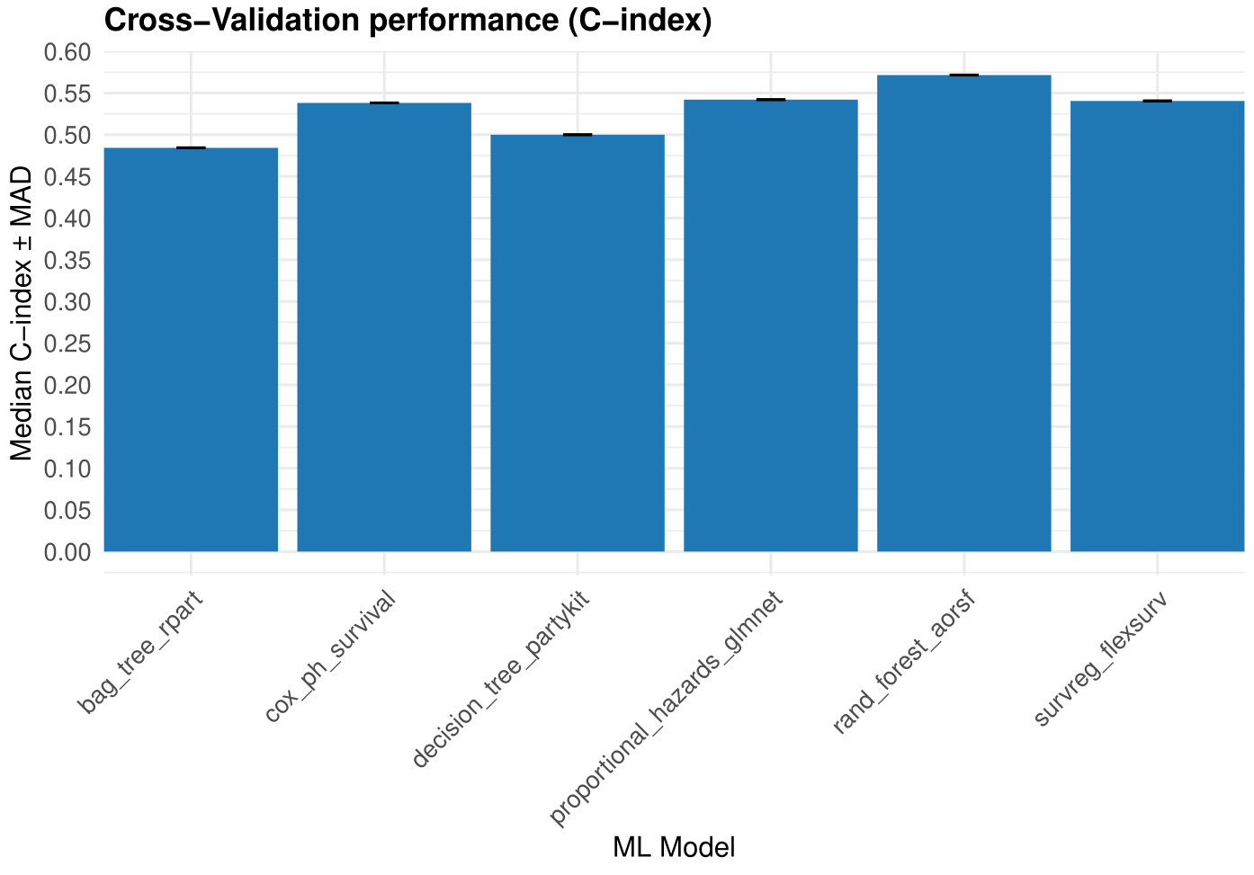
Figure 1. Cross-validation C-index of the trained models.

Predict on test data

pred_survival <- compute_prediction(model = res_survival$Model,
                                    test_data = X_test,
                                    task_type = "survival",
                                    time_var = time_test,
                                    event_var = event_test,
                                    file.name = "Example_survival",
                                    return = TRUE)

C-index on the test set, with its 95% confidence interval:

pred_survival$c_index
c(pred_survival$c_index_lower, pred_survival$c_index_upper)

Predicted risk scores of the test samples:

head(pred_survival$preds)

Depending on the model, survival models predict a linear predictor, a survival time or a survival probability. The modelling library (parsnip) returns all of them so that higher values mean longer survival. compute_prediction() reverses them into a risk score so that all models are read the same way:

• linear predictor (linear_pred), e.g. Cox models: parsnip returns it with the sign changed (higher = longer survival), so it is reversed back into a risk score;
• predicted survival time (time), e.g. tree-based models, is reversed: a longer survival means a lower risk;
• survival probability (survival) is also reversed: a higher probability of survival means a lower risk.

Higher prediction values always correspond to higher predicted risk.

Kaplan-Meier curves by risk group

With return = TRUE, compute_prediction() splits the test samples into two groups at the median predicted risk and saves their Kaplan-Meier curves in Results/ (Survival_KM_<file.name>.pdf), with the C-index and the log-rank test p-value. The High risk group contains the samples with the highest predicted risk scores, so its curve is expected to drop faster than the one of the Low risk group.

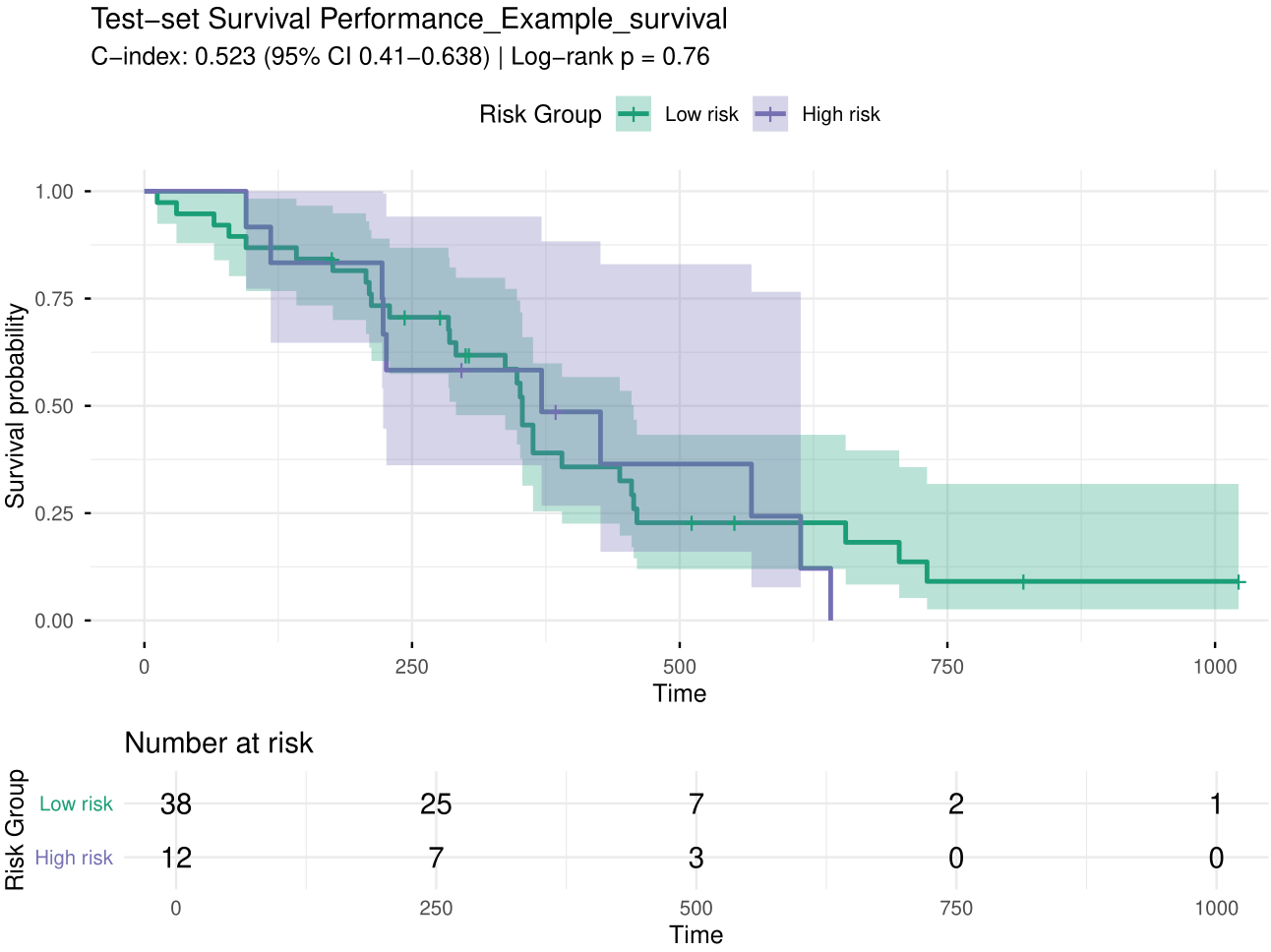
Figure 2. Kaplan-Meier curves of the test samples by predicted risk group (two groups).

The number of groups is set with n_groups (default 2). Groups are defined by quantiles of the predicted risk and are named Low/High risk (2 groups), Low/Medium/High risk (3 groups) or Group 1 (lowest risk) to Group n (highest risk):

pred_survival <- compute_prediction(model = res_survival$Model,
                                    test_data = X_test,
                                    task_type = "survival",
                                    time_var = time_test,
                                    event_var = event_test,
                                    file.name = "Example_survival_3groups",
                                    return = TRUE,
                                    n_groups = 3)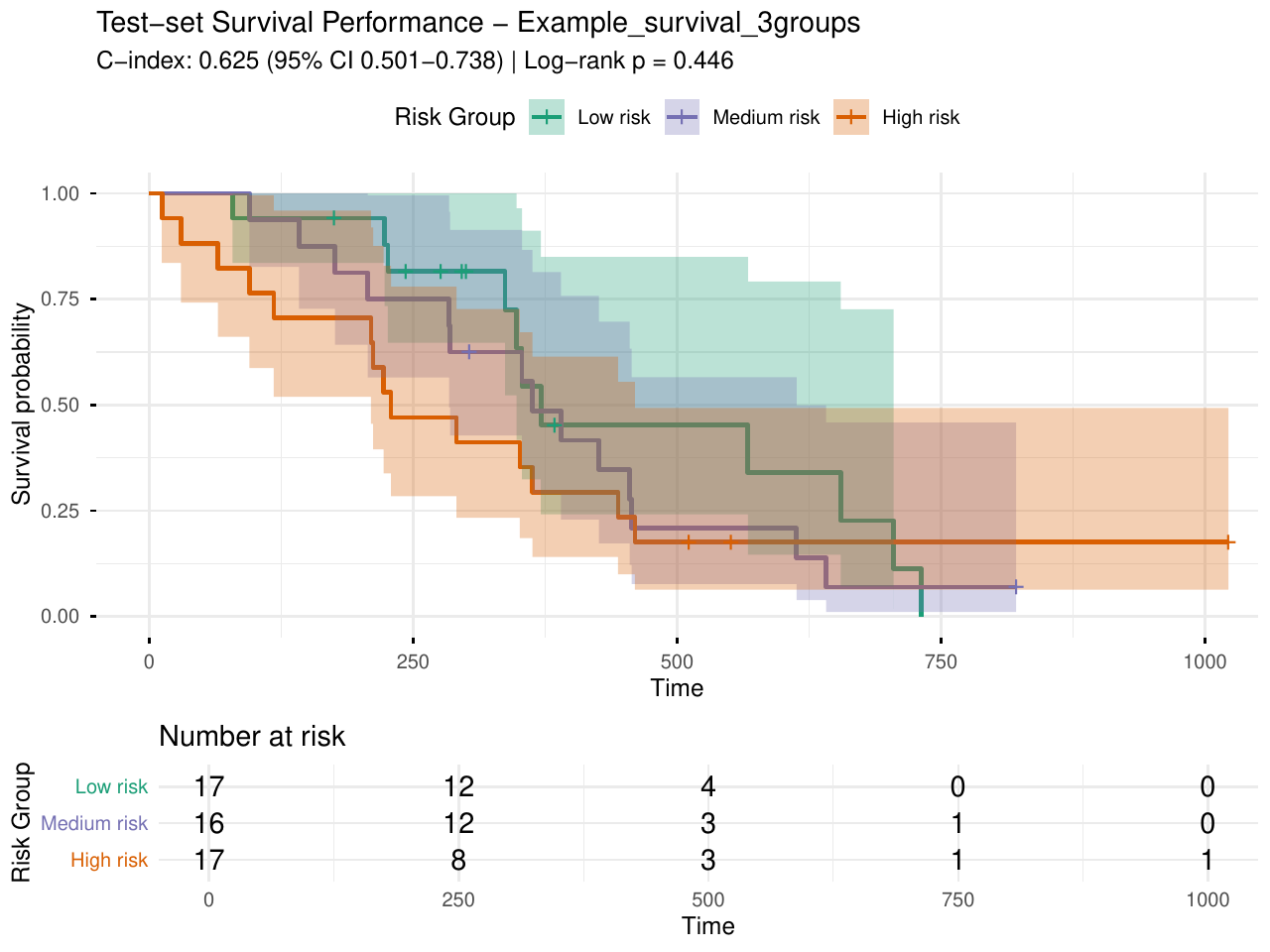

Figure 3. Kaplan-Meier curves of the test samples by predicted risk group (three groups).

The same plot can be drawn from an existing prediction with plot_survival_performance(), which takes the observed outcome of the test samples and the output of compute_prediction(). It returns the plot object, so it can be customized:

km <- plot_survival_performance(df_test = data.frame(time = time_test, event = event_test),
                                prediction = pred_survival,
                                n_groups = 3,
                                file_name = "Example_survival_3groups")
km$plot + ggplot2::labs(x = "Time (days)")

Some models (e.g. tree-based ones) predict only a few distinct risk scores. Samples with the same predicted risk are always kept in the same group, so the groups can have different sizes, and fewer groups than n_groups may be formed (a message says so).

SHAP values

compute_shap_values() works the same way as for classification, with task_type = "survival". SHAP values are in risk-score units: positive values push the prediction towards a higher risk.

shap_survival <- compute_shap_values(model_trained = res_survival$Model,
                                     task_type = "survival",
                                     seed = 123)
head(shap_survival)

Training and prediction in one step

compute_features.ML() trains and predicts in one step. For survival, time_var and event_var are the names of the time and event columns of coldata, whose row names must be the sample names of the feature tables:

res_onestep_survival <- compute_features.ML(features_train = X_train,
                                            features_test = X_test,
                                            coldata = data,
                                            task_type = "survival",
                                            time_var = "time",
                                            event_var = "status",
                                            k_folds = 3,
                                            n_rep = 1,
                                            ncores = 2,
                                            file_name = "Example_onestep_survival",
                                            return = FALSE)

res_onestep_survival$Model is the output of compute_features.training.ML(), C_index the C-index on the test set and Prediction the predicted risk scores:

res_onestep_survival$C_index
head(res_onestep_survival$Prediction)