pipeML
pipeML.Rmd
library(pipeML)
#> Warning: replacing previous import 'dplyr::explain' by 'fastshap::explain' when
#> loading 'pipeML'
library(caret)
#> Loading required package: ggplot2
#> Loading required package: lattice
library(dplyr)
#>
#> Attaching package: 'dplyr'
#> The following objects are masked from 'package:stats':
#>
#>     filter, lag
#> The following objects are masked from 'package:base':
#>
#>     intersect, setdiff, setequal, union
library(survival)
#>
#> Attaching package: 'survival'
#> The following object is masked from 'package:caret':
#>
#>     cluster
library(censored)
#> Loading required package: parsnip
library(doParallel)
#> Loading required package: foreach
#> Loading required package: iterators
#> Loading required package: parallel
This vignette demonstrates how to use pipeML to train,
tune, and evaluate machine learning models for classification and
survival tasks.
The content is organized into application-focused sections so you can jump directly to the workflow you need.
Get Started
pipeML provides two core workflows:
-
compute_features.training.ML(): train and tune models on a training set. -
compute_prediction(): evaluate trained models on a test set.
If you already have a test set prepared, you can also use:
-
compute_features.ML(): one-step training + prediction.
Classification and Survival
Classification Tasks
Load example data:
data = pipeML::data_example_classification
X <- data %>% dplyr::select(-target)
y <- data$target
For this example, make a train/test split:
set.seed(123)

train_idx <- caret::createDataPartition(y, p = 0.7, list = FALSE)

X_train <- X[train_idx, ]
X_test  <- X[-train_idx, ]

y_train <- y[train_idx]
y_test  <- y[-train_idx]
Train Models
Train and tune models using repeated stratified k-fold cross-validation:
res <- compute_features.training.ML(features_train = X_train,
                                    target_var = y_train,
                                    task_type = "classification",
                                    trait.positive = "1",
                                    metric = "AUROC",
                                    k_folds = 2,
                                    n_rep = 1,
                                    file_name = "Example_classification",
                                    return = F)
Access the best-trained model:
res$ModelView all trained and tuned machine learning models:
names(res$ML_Models)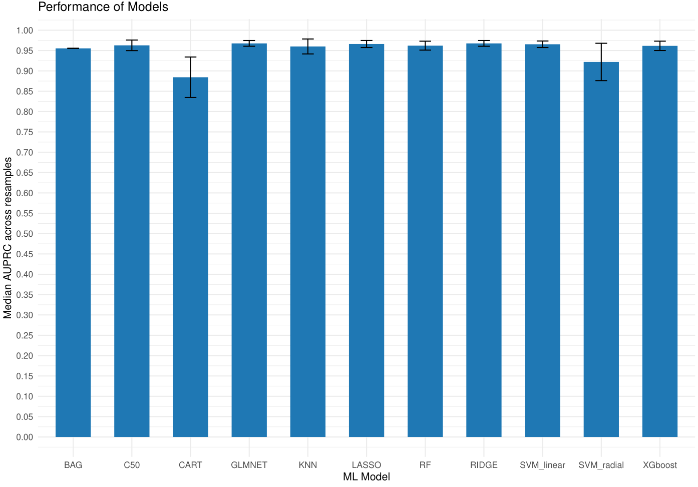
Figure 1. Models training performance.
Predict On Test Data
After training, users can predict on new data by using the
compute_prediction() function. You can specify which metric
to maximize when determining the optimal classification threshold.
Supported values for maximize include: “Accuracy”, “Precision”,
“Recall”, “Specificity”, “Sensitivity”, “F1”, and “MCC”.
pred = compute_prediction(model = res$Model,
                          test_data = X_test,
                          target_var = y_test,
                          task_type = "classification",
                          trait.positive = "1",
                          file.name = "Example_classification")
Check predictions:
head(pred$Predictions)Inspect threshold-based prediction metrics:
head(pred$Metrics)If return = TRUE, compute_prediction()
saves ROC and PR curves in the Results/ directory.
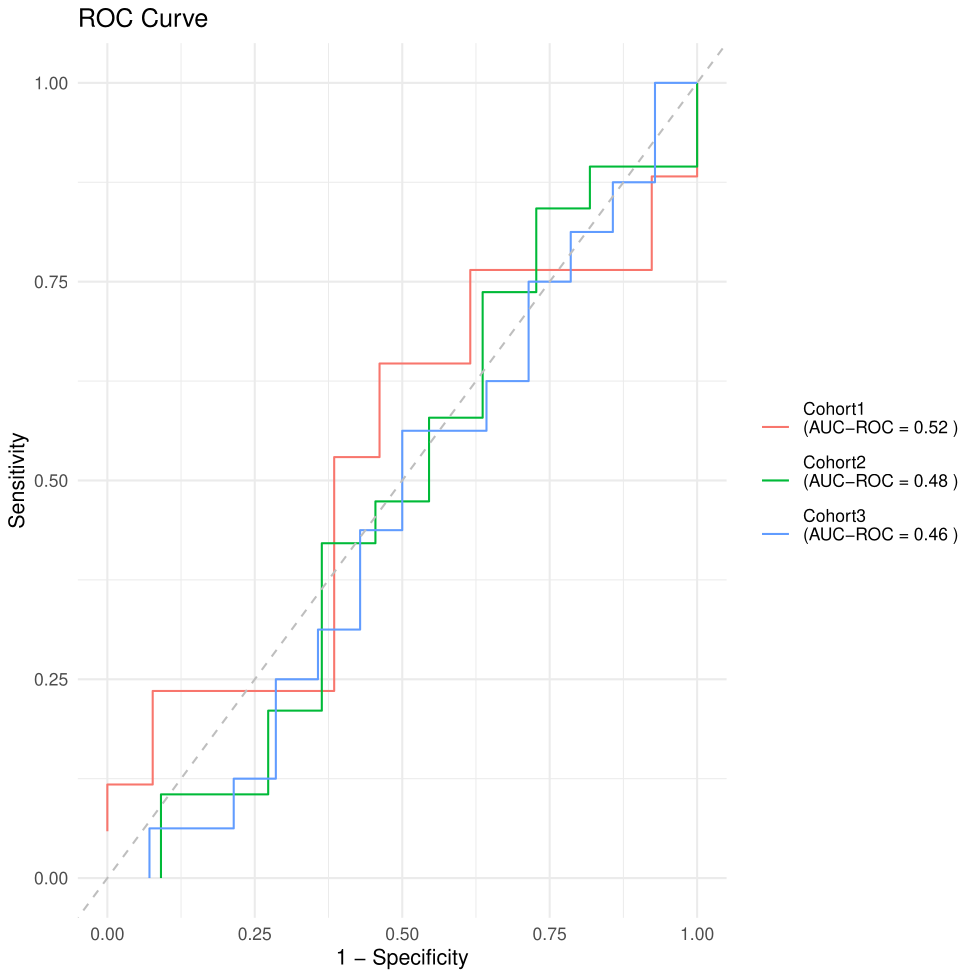
Figure 2. ROC curve.
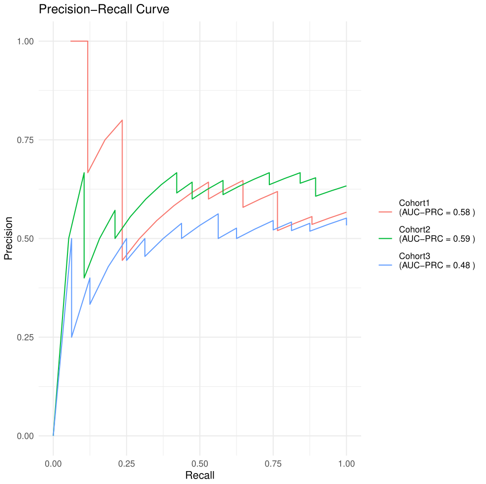
Figure 3. PR curve.
Compute SHAP Values
SHAP values help interpret machine learning predictions by quantifying feature contributions.
df = cbind(X_train, target = as.numeric(y_train)) ## compute_shap_values expects predictors and target in a single data.frame

shap_classification <- compute_shap_values(
  model_trained = res$Model,
  data_train = df,
  task_type = "classification",
  target_col = "target",
  trait.positive = "2", # Notice here that because of as.numeric() our target variable changed to 1 and 2 so we will consider 2 as our new 1.
  n_cores = 2,
  file.name = "Example_classification"
)
Visualize feature importance and interactions using shapviz:
sv <- shapviz::shapviz(
  shap = as.matrix(shap_classification$shap_values),
  X = df[, setdiff(colnames(df), "target")]
)

# Global feature importance (bar plot)
shapviz::sv_importance(sv, kind = "bar") +
  ggplot2::ggtitle("Global Feature Importance")

# Beeswarm plot
shapviz::sv_importance(sv, kind = "beeswarm") +
  ggplot2::ggtitle("SHAP Beeswarm Summary")

# Feature dependence plots for top 6 features
top_features <- names(sort(colMeans(abs(shap_classification$shap_values)), decreasing = TRUE))[1:6]

for (f in top_features) {
  print(
    shapviz::sv_dependence(sv, v = f) +
    ggplot2::ggtitle(paste0("Dependence: ", f))
  )
}
Model Stacking
To apply model stacking, set stack = TRUE:
res <- compute_features.training.ML(features_train = X_train,
                                    target_var = y_train,
                                    task_type = "classification",
                                    trait.positive = "1",
                                    metric = "AUROC",
                                    stack = T,
                                    k_folds = 2,
                                    n_rep = 1,
                                    file_name = "Example_classification",
                                    return = F)
Survival Tasks
In addition to classification and regression tasks,
pipeML supports survival analysis, allowing users to train
machine learning models that predict time-to-event outcomes.
In survival analysis, the response variable is defined by two components:
- Time: follow-up or survival time
- Event: indicator of whether the event occurred (1) or the observation was censored (0)
pipeML automates the training, evaluation, and
interpretation of survival models using cross-validation and SHAP-based
explanations.
Load example dataset for survival:
data = pipeML::data_example_survival
X <- data %>% dplyr::select(-time, -status)
time <- data$time
event <- data$status
Similar to the previous example, split data into train/test:
set.seed(123)
train_idx <- caret::createDataPartition(event, p = 0.7, list = FALSE)

X_train <- X[train_idx, ]
X_test  <- X[-train_idx, ]

time_train <- time[train_idx]
time_test  <- time[-train_idx]

event_train <- event[train_idx]
event_test  <- event[-train_idx]
Train Models
The function compute_features.training.ML() can also
train survival models by setting
task_type = "survival".
res_survival <- compute_features.training.ML(
  features_train = X_train,
  task_type = "survival",
  time_var = time_train,
  event_var = event_train,
  k_folds = 2,
  n_rep = 1,
  file_name = "Example_survival",
  ncores = 1
)
Access the best model:
names(res_survival$ML_Models)
res_survival$Model$Model_object
Check training metrics:
head(res_survival$Model$Prediction_folds)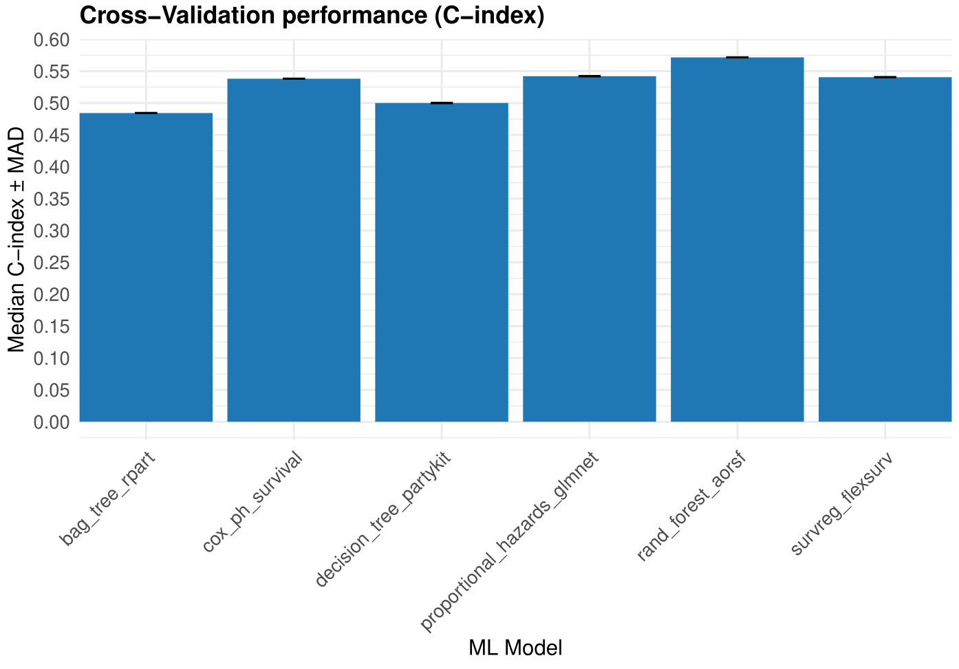
Figure 4. Models training performance.
Predict On Test Data
After training, predictions can be generated using
compute_prediction().
pred <- compute_prediction(
  model = res_survival$Model,
  test_data = X_test,
  task_type = "survival",
  time_var = time_test,
  event_var = event_test,
  file.name = "Example_survival")
Unlike classification models, survival models may return different types of predictions depending on the model used. Some models predict a risk score, while others predict expected survival time or survival probability.
The compute_prediction() function automatically handles
these differences. Internally, it attempts several prediction types and
converts them into a standardized risk score so that results can be
compared across models:
- Risk score (linear_pred) – typically produced by Cox models. Higher values indicate higher predicted risk.
- Predicted survival time (time) – produced by some parametric survival models. Higher values indicate longer survival, so the values are internally reversed to represent risk.
- Survival probability (survival) – probability of surviving at a given time point. Higher probabilities correspond to lower risk, so these values are also internally reversed.
After this standardization step, predictions are always interpreted in the same way:
Higher prediction values correspond to higher predicted risk
This allows pipeML to compute performance metrics such
as the concordance index (C-index) and to stratify patients into risk
groups for Kaplan–Meier visualization.
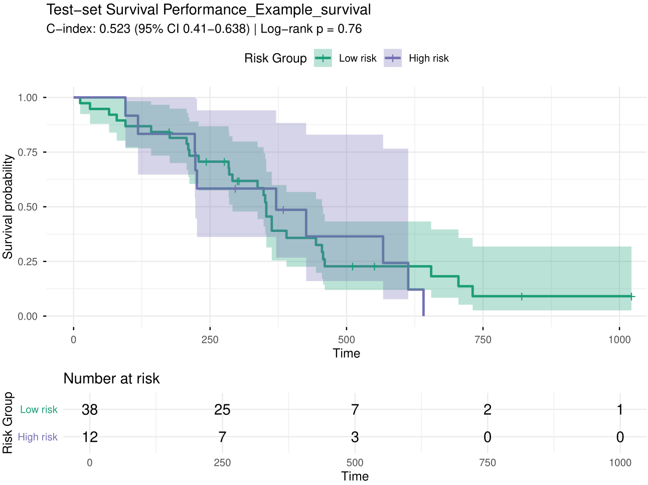
Figure 5. KM plot.
Compute SHAP Values
We will use the same function compute_shap_values
computed before but this time with the
task_type = "survival".
shap_survival <- compute_shap_values(
  model_trained = res_survival$Model,
  data_train = df,
  task_type = "survival",
  time_col = "time",
  event_col = "status",
  n_cores = 2,
  file.name = "Example_survival"
)
One-Step Training and Prediction
If a separate testing dataset is already available,
pipeML allows you to train models and generate predictions
in a single step using the compute_features.ML() function.
This function performs model training, hyperparameter tuning, and
evaluation on the training data, and then applies the selected model to
the test dataset.
Classification Example
data = pipeML::data_example_classification
X <- data %>% dplyr::select(-target)
y <- data$target

set.seed(123)

train_idx <- caret::createDataPartition(y, p = 0.8, list = FALSE)

X_train <- X[train_idx, ]
X_test  <- X[-train_idx, ]
res <- compute_features.ML(features_train = X_train,
                           features_test = X_test,
                           coldata = data,
                           task_type = "classification",
                           trait = "target",
                           trait.positive = "1",
                           metric = "AUROC",
                           k_folds = 2,
                           n_rep = 1,
                           ncores = 2,
                           file_name = "Test",
                           return = FALSE)
Survival Example
data = pipeML::data_example_survival
X <- data %>% dplyr::select(-time, -status)
time <- data$time
event <- data$status

set.seed(123)
train_idx <- caret::createDataPartition(event, p = 0.7, list = FALSE)

X_train <- X[train_idx, ]
X_test  <- X[-train_idx, ]

time_train <- time[train_idx]
time_test  <- time[-train_idx]

event_train <- event[train_idx]
event_test  <- event[-train_idx]
res <- compute_features.ML(features_train = X_train,
                           features_test = X_test,
                           coldata = data,
                           task_type = "survival",
                           time_var = "time",
                           event_var = "status",
                           k_folds = 2,
                           n_rep = 1,
                           ncores = 2,
                           file_name = "Test",
                           return = FALSE)
Advanced
Leave-One-Dataset-Out (LODO) Analysis
If your data includes features from multiple cohorts,
pipeML provides a flexible approach to perform
Leave-One-Dataset-Out (LODO) analysis. This is achieved
by applying k-fold stratified sampling across batches, ensuring that
each fold preserves the batch structure while maintaining class balance.
To enable this, set LODO = TRUE and provide the column name
containing batch information in batch_var.
Below, we demonstrate how to perform a LODO analysis using simulated datasets:
Simulate datasets from different batches (‘cohorts’)
set.seed(123)

# Simulate traitData with 3 cohorts
traitData <- data.frame(
  Sample = paste0("Sample", 1:90),
  Response = sample(c("R", "NR"), 90, replace = TRUE),
  Cohort = rep(paste0("Cohort", 1:3), each = 30),
  stringsAsFactors = FALSE
)
rownames(traitData) <- traitData$Sample

# Simulate counts matrix
counts_all <- matrix(rnorm(1000 * 90), nrow = 1000, ncol = 90)
rownames(counts_all) <- paste0("Gene", 1:1000)
colnames(counts_all) <- traitData$Sample

# Simulate some example features
features_all <- matrix(runif(90 * 15), nrow = 90, ncol = 15)
rownames(features_all) <- traitData$Sample
colnames(features_all) <- paste0("Feature", 1:15)
Perform LODO analysis using base function
compute_features.training.ML
prediction = list()
i = 1
for (cohort in unique(traitData$Cohort)) {

  # Test cohort
  traitData_test = traitData %>%
    filter(Cohort == cohort)
  counts_test = counts_all[,colnames(counts_all)%in%rownames(traitData_test)]
  features_test = features_all[rownames(features_all)%in%rownames(traitData_test),]

  # Train cohort
  traitData_train = traitData %>%
    filter(Cohort != cohort)
  counts_train = counts_all[,colnames(counts_all)%in%rownames(traitData_train)]
  features_train = features_all[rownames(features_all)%in%rownames(traitData_train),]

  #### ML Training
  res = compute_features.training.ML(features_train = features_train,
                                     target_var = traitData_train$Response,
                                     task_type = "classification",
                                     trait.positive = "R",
                                     metric = "AUROC",
                                     k_folds = 2,
                                     n_rep = 1,
                                     LODO = TRUE,
                                     batch_var = traitData_train$Cohort,
                                     ncores = 1,
                                     return = F)

  #### ML predicting

  #### Testing
  pred = compute_prediction(model = res$Model,
                            test_data = features_test,
                            target_var = traitData_test$Response,
                            task_type = "classification",
                            trait.positive = "R",
                            return = F)

  #### Save results
  prediction[[i]] = pred
  names(prediction)[i] = cohort
  i = i + 1
}
For plotting, we use get_curves(), adapted for multiple
cohorts. This function is used internally by
compute_prediction() to generate ROC and PR curves.
Extract prediction metrics and join
roc_data <- lapply(names(prediction), function(cohort) {
  df <- prediction[[cohort]]$Metrics
  df$cohort <- cohort
  df
}) %>% dplyr::bind_rows()

auc_roc <- list(
  mean  = sapply(prediction, function(x) x$AUC$AUROC$mean),
  lower = sapply(prediction, function(x) x$AUC$AUROC$lower),
  upper = sapply(prediction, function(x) x$AUC$AUROC$upper)
)

auc_prc <- list(
  mean  = sapply(prediction, function(x) x$AUC$AUPRC$mean),
  lower = sapply(prediction, function(x) x$AUC$AUPRC$lower),
  upper = sapply(prediction, function(x) x$AUC$AUPRC$upper)
)
Plot ROC and PR curves:
get_curves(
  data = roc_data,
  color = "cohort",
  auc_roc = auc_roc,
  auc_prc = auc_prc,
  LODO = TRUE,
  file.name = "LODO_cohort_example",
  width = 9,
  height = 9
)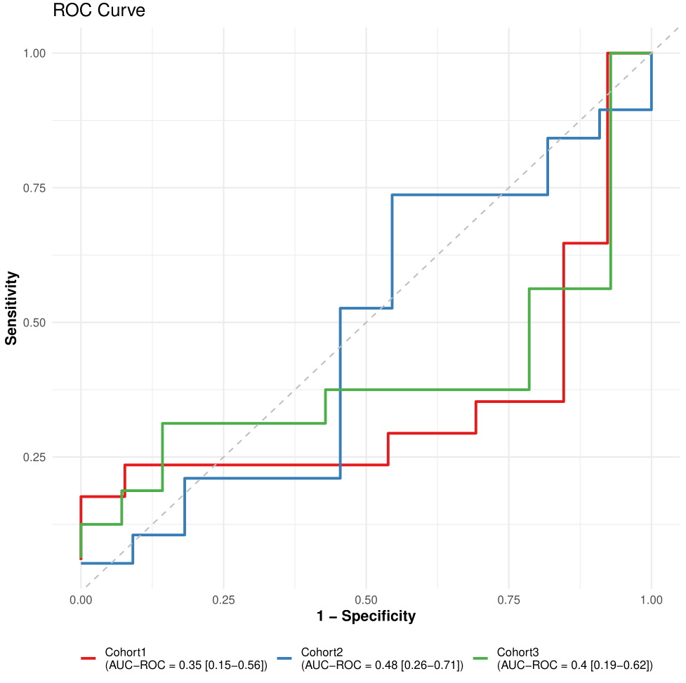
Figure 6. LODO ROC curves.
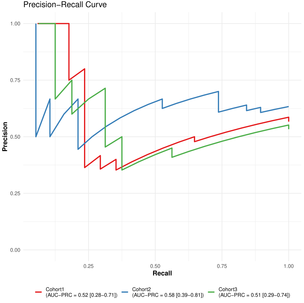
Figure 7. LODO PR curves.
Leakage-Aware Custom Cross-Validation
A central design principle of pipeML is to prevent
information leakage during model training and evaluation. In many
machine learning workflows, feature engineering steps are applied to the
full dataset before cross-validation, which can inadvertently introduce
information from the test folds into the training process. This leads to
overoptimistic performance estimates.
To address this, pipeML provides built-in support for
custom fold construction through the fold_construction_fun
argument in compute_features.training.ML(). This mechanism
allows feature engineering and preprocessing steps to be recomputed
independently within each cross-validation fold, ensuring that test
samples never influence the training process.
This capability is a core component of the pipeML
pipeline, enabling leakage-aware model development for
datasets where features depend on the full sample structure.
Why custom fold construction is important?
In many biological and high-dimensional datasets, features are not independent variables but are derived from the data itself. Examples include:
- correlation-based clustering
- dimensionality reduction (e.g., PCA)
- gene set enrichment or pathway scoring
- transcription factor activity inference
- aggregation of features across samples
If these transformations are applied to the entire dataset before cross-validation, the test samples influence how the feature space is constructed. As a result, the model indirectly “sees” information from the test data during training.
By recomputing these steps within each fold, pipeML
ensures that:
- training data are used to define the feature space
- test samples are projected onto the learned space without influencing it
- model evaluation reflects true out-of-sample performance
This approach closely mimics how the model would behave when applied to completely unseen data, producing more realistic performance estimates.
Step 1 - Define a base feature function (e.g. WGCNA)
Structure of the Base Feature Function
The function is designed around two operational modes:
- Training Mode (modules is NULL): The function learns the feature structure from the input dataset.
- Projection Mode (modules provided): The function applies a previously learned structure to new data.
Why the Function Returns Two Objects?
- features → always returned; the transformed representation of the current dataset (training or test).
- structure → returned only when learning from training data; needed to project test data in future steps.
This ensures a leakage-aware workflow:
- Training data defines the feature space.
- Test data is projected without altering the learned structure.
Structure of base function
- data: features as rows, samples as columns
-
structure: precomputed structure (e.g., clusters,
components);
NULLfor training - …: additional arguments specific to the algorithm used
compute_features_modular <- function(data, structure = NULL, ...) {


  # TRAINING MODE
  if (is.null(structure)) {

    # -------------------- REPLACE THIS BLOCK --------------------
    structure <- learn_structure(data, ...) # user-defined function
    # -------------------- REPLACE THIS BLOCK --------------------

  }

  # PROJECT MODE

  # -------------------- REPLACE THIS BLOCK --------------------
  features <- project_data(data, structure, ...) # user-defined function
  # -------------------- REPLACE THIS BLOCK --------------------


  return(list(features = features, structure = structure))
}
Here we illustrate a correlation-based feature computation using Weighted Gene Co-expression Network Analysis (WGCNA). This is just an example: in practice, you can use any feature computation that depends on multiple samples, such as clustering, PCA, among others.
library(WGCNA)
compute_features_modular <- function(counts, power = NULL, modules = NULL) {

  ## Just preprocessing (IGNORE)
  rownames(counts) <- gsub("-", ".", rownames(counts))
  datExpr <- t(counts)
  cor <- WGCNA::cor

  # TRAINING MODE
  if (is.null(modules)) {

    # -------------------- REPLACE THIS BLOCK --------------------
    net <- WGCNA::blockwiseModules(datExpr, power = power)
    modules <- net$colors
    names(modules) <- colnames(datExpr)
    # -------------------- REPLACE THIS BLOCK --------------------

  }

  # PROJECT MODE

  # -------------------- REPLACE THIS BLOCK --------------------
  module_features <- sapply(unique(modules), function(mod) {
    genes <- names(modules[modules == mod])
    pc <- prcomp(datExpr[, genes, drop = FALSE])
    pc$x[, 1]
  })
  # -------------------- REPLACE THIS BLOCK --------------------

  ## Just formatting (IGNORE)
  colnames(module_features) <- paste0("Module_", seq_len(ncol(module_features)))


  return(list(features = as.matrix(module_features), structure = modules))
}
Step 2 - Make the function suitable for pipeML
We then need to extend and give the correct format to this function
to make it suitable for running across folds inside
pipeML
This template provides a modular framework to prepare
cross-validation folds for pipeML in a leakage-aware way.
It separates training vs projection:
- Training mode: computes features and learns the data structure from the training folds
- Projection mode: applies the learned structure to held-out folds without influencing it.
Users can easily adapt this template by replacing their previous
compute_features_modular function
NOTE
In pipeML data corresponds to samples as rows and
features as columns. If your compute_features_modular()
needs features as rows, make sure to t() inside this
function.
The parameters data, folds, and
bestune are handled by pipeML automatically
once fold_construction_fun is set. Do not change these
parameter names or remove them.
- … : Additional parameters passed to your feature function
Make sure compute_features_modular() returns a matrix
with the features. If not, make sure to extract them before adding the
target column
prepare_custom_folds <- function(data, folds = NULL, bestune = NULL, ...) {

  if (!is.null(bestune)) {

    obs_train <- data$target
    data$target <- NULL


    # -------------------- REPLACE THIS BLOCK --------------------
    result <- compute_features_modular(data, ...)
    # -------------------- REPLACE THIS BLOCK --------------------


    train_features_final = result$features
    train_features_final$target <- obs_train

    custom_output <- result

    return(list(train_features_final, custom_output, bestune))

  } else {

    processed_folds <- list()

    for (i in seq_along(folds)) {

      train_idx <- folds[[i]]
      test_idx  <- setdiff(seq_len(nrow(data)), train_idx)

      train_data <- data[train_idx, , drop = FALSE]
      obs_train <- train_data$target
      train_data$target <- NULL


      # -------------------- REPLACE THIS BLOCK --------------------
      train_result <- compute_features_modular(train_data, ...)
      # -------------------- REPLACE THIS BLOCK --------------------


      train_features = train_result$features
      train_features$target <- obs_train

      test_data <- data[test_idx, , drop = FALSE]
      obs_test <- test_data$target
      test_data$target <- NULL


      # -------------------- REPLACE THIS BLOCK --------------------
      test_features <- compute_features_modular(
        test_data,
        structure = train_result$structure,
        ...
      )
      # -------------------- REPLACE THIS BLOCK --------------------


      test_features = test_features$features

      processed_folds[[i]] <- list(
        train_data = train_features,
        test_data  = test_features,
        obs_test   = obs_test,
        rowIndex   = test_idx,
        fold_name  = names(folds)[i]
      )
    }

    for (i in seq_along(processed_folds)) {
      filename <- file.path("Results", paste0("fold_", names(folds)[i], ".rds"))
      saveRDS(processed_folds[[i]], file = filename)
    }

    return(processed_folds)
  }
}
Here we illustrate how the function will look applying our
compute_features_modular() function
Notice that each time I call the function
compute_features_modular() I am setting my additional
argument power
prepare_WGCNA_folds <- function(data, folds = NULL, bestune = NULL, power) {

  if (!is.null(bestune)) {

    obs_train <- data$target
    data$target <- NULL


    # -------------------- REPLACE THIS BLOCK --------------------
    wgcna_result <- compute_features_modular(t(data), power = power)
    # -------------------- REPLACE THIS BLOCK --------------------


    train_cell_data_final <- as.data.frame(wgcna_result$features)
    train_cell_data_final$target <- obs_train

    custom_output <- wgcna_result

    return(list(train_cell_data_final, custom_output, bestune))

  } else {

    processed_folds <- list()

    for (i in seq_along(folds)) {

      train_idx <- folds[[i]]
      test_idx  <- setdiff(seq_len(nrow(data)), train_idx)

      train_data <- data[train_idx, , drop = FALSE]
      obs_train <- train_data$target
      train_data$target <- NULL


      # -------------------- REPLACE THIS BLOCK --------------------
      train_result <- compute_features_modular(t(train_data), power = power)
      # -------------------- REPLACE THIS BLOCK --------------------


      train_features <- as.data.frame(train_result$features)
      train_features$target <- obs_train

      test_data <- data[test_idx, , drop = FALSE]
      obs_test <- test_data$target
      test_data$target <- NULL


      # -------------------- REPLACE THIS BLOCK --------------------
      test_features <- compute_features_modular(t(test_data),
                                                modules = train_result$structure)
      # -------------------- REPLACE THIS BLOCK --------------------


      test_features <- as.data.frame(test_features$features)

      processed_folds[[i]] <- list(
        train_data = train_features,
        test_data  = test_features,
        obs_test   = obs_test,
        rowIndex   = test_idx,
        fold_name  = names(folds)[i]
      )
    }

    for (i in seq_along(processed_folds)) {
      filename <- file.path("Results", paste0("fold_", names(folds)[i], ".rds"))
      saveRDS(processed_folds[[i]], file = filename)
    }

    return(processed_folds)
  }
}
Load data example
counts = pipeML::counts_example
coldata = pipeML::coldata_example

set.seed(123)

train_idx <- caret::createDataPartition(coldata$Response, p = 0.7, list = FALSE)

counts_train <- counts[, train_idx]
counts_test  <- counts[, -train_idx]

coldata_train <- coldata[train_idx,]
coldata_test  <- coldata[-train_idx,]
Step 3 - Run custom k-fold cross-validation
Once your custom fold function is ready, pass it to
compute_features.training.ML() via
fold_construction_fun.
Note the argument fold_construction_args_fixed
corresponds to the additional parameters passed in
prepare_custom_folds() function (in this example
prepare_WGCNA_folds()). They should be set with the value
to use when running your function. If your function does not have any
parameters, you can ignore this argument and it will be set up to
NULL.
res_custom   = compute_features.training.ML(features_train = t(counts_train),
                                            target_var     = coldata_train$Response,
                                            task_type      = "classification",
                                            trait.positive = "R",
                                            metric         = "AUROC",
                                            k_folds        = 2,
                                            n_rep          = 1,
                                            return         = FALSE,
                                            fold_construction_fun = prepare_WGCNA_folds,
                                            fold_construction_args_fixed = list(power=6))
Notice that res_custom$Custom_output contains the output
features of your base function in case these are needed (e.g. for
prediction - see next section)
Step 4 - Tunable hyperparameters within custom fold functions (optional)
In some scenarios, the feature construction step may include
parameters whose values can influence model performance. For example,
when computing WGCNA, parameters such as
soft-thresholding power, minimum module size,
module merging threshold, and
module splitting sensitivity may affect the resulting
features and therefore the downstream model performance.
To address this, pipeML supports hyperparameter tuning
within your custom fold functions. This allows users to identify which
parameter values lead to the best predictive performance.
Briefly, the user provides a grid of candidate parameter values, and
pipeML will:
- construct custom cross-validation folds for each parameter combination
- train and evaluate machine learning models for each configuration
- compare the resulting performance across folds and repetitions
- return the parameter values that maximize the selected performance metric
Before that, user needs to modify
compute_features_modular and
prepare_custom_folds() to account for all these
parameters.
For the compute_features_modular we are only going to
add the tunable parameters in our function call
compute_features_modular <- function(
    counts,
    power = NULL,
    modules = NULL,
    ## tunable parameters
    minModuleSize,
    mergeCutHeight,
    deepSplit
) {

  ## Just preprocessing (IGNORE)
  rownames(counts) <- gsub("-", ".", rownames(counts))
  datExpr <- t(counts)
  cor <- WGCNA::cor

  # TRAINING MODE

  if (is.null(modules)) {


    # -------------------- REPLACE THIS BLOCK --------------------
    net <- WGCNA::blockwiseModules(
      datExpr,
      power = power,
      minModuleSize = minModuleSize,
      mergeCutHeight = mergeCutHeight,
      deepSplit = deepSplit
    )
    modules <- net$colors
    names(modules) <- colnames(datExpr)
    # -------------------- REPLACE THIS BLOCK --------------------


  }

  # PROJECT MODE


  # -------------------- REPLACE THIS BLOCK --------------------
  module_features <- sapply(unique(modules), function(mod) {
    genes <- names(modules[modules == mod])
    pc <- prcomp(datExpr[, genes, drop = FALSE])
    pc$x[, 1]
  })
  # -------------------- REPLACE THIS BLOCK --------------------


  ## Just formatting (IGNORE)
  colnames(module_features) <- paste0("Module_", seq_len(ncol(module_features)))

  return(list(features = as.matrix(module_features), structure = modules))
}
Then we will use this version of prepare_custom_folds()
that have some modifications to account for parameters combinations
Notice we have an additional parameter ncores that
controls parallelization when evaluating all runs (do not remove
it!).
prepare_custom_folds_tuning <- function(data,
                                        folds = NULL,
                                        bestune = NULL,
                                        ncores = NULL, ...){

  if (!is.null(bestune)) {

    obs_train <- data$target
    data$target <- NULL

    # -------------------- REPLACE THIS BLOCK --------------------
    required_cols <- c()# list your params separated by a comma
    # -------------------- REPLACE THIS BLOCK --------------------

    best_params <- if (is.data.frame(bestune)) {
      if (all(required_cols %in% names(bestune))) {
        dplyr::select(bestune, dplyr::all_of(required_cols))
      }else{stop("Not all tunable params found. Verify your function.")}
    } else if (is.list(bestune)) {
      if (all(required_cols %in% names(bestune))) {
        tibble::as_tibble(bestune[required_cols])
      }else{stop("Not all tunable params found. Verify your function.")}
    } else {
      stop("`bestune` must be a data.frame or list.")
    }


    # -------------------- REPLACE THIS BLOCK --------------------
    res_final <- compute_features_modular(
      counts = data,
      # change param1, param2, ... for the names of your parameters
      param1 = best_params$param1,
      param2 = best_params$param2,
      param3 = best_params$param3
      ...
    )
    # -------------------- REPLACE THIS BLOCK --------------------


    train_features_final = res_final$features
    train_features_final$target <- obs_train

    custom_output <- res_final

    return(list(train_features_final, custom_output, bestune))

  } else {


    # -------------------- REPLACE THIS BLOCK --------------------
    custom_grid <- expand.grid(
      param1 = param1,
      param2 = param2,
      param3 = param3,
      ...,
      stringsAsFactors = FALSE
    )
    # -------------------- REPLACE THIS BLOCK --------------------


    if (is.null(ncores)) ncores <- parallel::detectCores() - 2
    cl <- parallel::makeCluster(ncores)
    doParallel::registerDoParallel(cl)

    processed_folds <- foreach::foreach(i = seq_along(folds),
                                        .packages = c("dplyr"),
                                        .export = c("compute_features_modular")
                                       ) %dopar% {

      train_idx <- folds[[i]]
      test_idx  <- setdiff(seq_len(nrow(data)), train_idx)

      train_data <- data[train_idx, , drop = FALSE]
      obs_train <- train_data$target
      train_data$target <- NULL

      fold_results <- lapply(seq_len(nrow(param_grid)), function(j) {
        params <- param_grid[j, ]


        # -------------------- REPLACE THIS BLOCK --------------------
        res_train <- compute_features_modular(
          counts = train_data,
          param1 = params$param1,
          param2 = params$param2,
          param3 = params$param3,
          ...
        )
        # -------------------- REPLACE THIS BLOCK --------------------


        train_features <- as.data.frame(res_train$features)
        train_features$target <- obs_train

        test_data <- data[test_idx, , drop = FALSE]
        obs_test <- test_data$target
        test_data$target <- NULL


        # -------------------- REPLACE THIS BLOCK --------------------
        test_features <- compute_features_modular(
          test_data,
          structure = res_train$structure,
          ...
        )
        # -------------------- REPLACE THIS BLOCK --------------------


        test_features = test_features$features

        list(
          train_data = train_features,
          test_data  = test_features,
          obs_test   = obs_test,
          rowIndex   = test_idx,
          fold_name  = names(folds)[i],
          params     = params
        )
      })

      filename <- file.path("Results", paste0("fold_", names(folds)[i], ".rds"))
      saveRDS(processed_folds[[i]], file = filename)

      fold_results

    }

    parallel::stopCluster(cl)
    foreach::registerDoSEQ()
    gc()

  }
}
In our case it would be:
prepare_WGCNA_folds_modular <- function(
    data,
    folds = NULL,
    bestune = NULL,
    power = NULL,
    ncores = NULL,
    ### tunable parameters
    minModuleSize,
    mergeCutHeight,
    deepSplit
) {

  if (!is.null(bestune)) {

    obs_train <- data$target
    data$target <- NULL


    # -------------------- REPLACE THIS BLOCK --------------------
    required_cols <- c("minModuleSize", "mergeCutHeight", "deepSplit")
    # -------------------- REPLACE THIS BLOCK --------------------


    best_params <- if (is.data.frame(bestune)) {
      if (all(required_cols %in% names(bestune))) {
        dplyr::select(bestune, dplyr::all_of(required_cols))
      }else{stop("Not all tunable params found. Verify your function.")}
    } else if (is.list(bestune)) {
      if (all(required_cols %in% names(bestune))) {
        tibble::as_tibble(bestune[required_cols])
      }else{stop("Not all tunable params found. Verify your function.")}
    } else {
      stop("`bestune` must be a data.frame or list.")
    }


    # -------------------- REPLACE THIS BLOCK --------------------
    res_final <- compute_features_modular(
      counts = t(data),
      power = power,
      ## tunable parameters
      minModuleSize = best_params$minModuleSize,
      mergeCutHeight = best_params$mergeCutHeight,
      deepSplit = best_params$deepSplit
    )
    # -------------------- REPLACE THIS BLOCK --------------------


    train_cell_data_final <- as.data.frame(res_final$features)
    train_cell_data_final$target <- obs_train

    custom_output <- res_final

    return(list(train_cell_data_final, custom_output, best_params))

  } else {


    # -------------------- REPLACE THIS BLOCK --------------------
    custom_grid <- expand.grid(
      minModuleSize = minModuleSize,
      mergeCutHeight = mergeCutHeight,
      deepSplit = deepSplit,
      stringsAsFactors = FALSE
    )
    # -------------------- REPLACE THIS BLOCK --------------------


    if (is.null(ncores)) ncores <- parallel::detectCores() - 2
    cl <- parallel::makeCluster(ncores)
    doParallel::registerDoParallel(cl)

    processed_folds <- foreach::foreach(i = seq_along(folds),
                                        .packages = c("dplyr"),
                                        .export = c("compute_features_modular")
                                        ) %dopar% {

      train_idx <- folds[[i]]
      test_idx <- setdiff(seq_len(nrow(data)), train_idx)

      train_data <- data[train_idx, , drop = FALSE]
      obs_train <- train_data$target
      train_data$target <- NULL

      fold_results <- lapply(seq_len(nrow(custom_grid)), function(j) {

        params <- custom_grid[j, ]


        # -------------------- REPLACE THIS BLOCK --------------------
        wgcna_train <- compute_features_modular(
          counts = t(train_data),
          power = power,
          ## tunable parameters
          minModuleSize = params$minModuleSize,
          mergeCutHeight = params$mergeCutHeight,
          deepSplit = params$deepSplit
        )
        # -------------------- REPLACE THIS BLOCK --------------------


        train_features <- as.data.frame(wgcna_train$features)
        train_features$target <- obs_train

        test_data <- data[test_idx, , drop = FALSE]
        obs_test <- test_data$target
        test_data$target <- NULL


        # -------------------- REPLACE THIS BLOCK --------------------
        wgcna_test <- compute_features_modular(
          counts = t(test_data),
          modules = wgcna_train$structure
        )
        # -------------------- REPLACE THIS BLOCK --------------------


        test_features <- as.data.frame(wgcna_test$features)

        list(
          train_data = train_features,
          test_data = test_features,
          obs_test = obs_test,
          rowIndex = test_idx,
          fold_name = names(folds)[i],
          params = params
        )
      })

      filename <- file.path("Results", paste0("fold_", names(folds)[i], ".rds"))
      saveRDS(fold_results, file = filename)

      fold_results
    }

    parallel::stopCluster(cl)
    foreach::registerDoSEQ()
    gc()

  }
}
To enable this functionality, the user must specify the argument
fold_construction_args_tunable, which contains the set of
parameter values to be evaluated
Note the argument fold_construction_args_fixed
corresponds to the additional parameters passed in
prepare_custom_folds() function that are not tunable (in
our case power and ncores). This means these
parameters are going to have the same value across all runs
(fix). Be sure of setting ncores to a
value that your computer can handle to avoid crashing.
The tunable parameters define the search space explored during feature computation. The total number of configurations corresponds to all combinations of the provided parameter values. In this example:
-
minModuleSize= c(20, 50, 100) → 3 values -
mergeCutHeight= c(0.15, 0.25, 0.35) → 3 values -
deepSplit= c(1, 2, 3) → 3 values
This results in 3 × 3 × 3 = 27 feature parameter combinations.
For each of these 27 configurations, the machine learning models are
trained and tuned. For example, if logistic regression with elastic net
(glmnet) is used, the model internally evaluates different
values of the hyperparameters alpha and
lambda. If the model tests 10 alpha values and 20
lambda values, this results in 200 model
configurations for each feature combination.
Therefore, the total number of evaluated models becomes:
27 (feature configurations) × 200 (model hyperparameter combinations) = 5400 model fits, which are further multiplied by the number of folds and repetitions used in cross-validation.
res_params <- compute_features.training.ML(features_train = t(counts_train),
                                           target_var     = coldata_train$Response,
                                           task_type = "classification",
                                           trait.positive = "R",
                                           metric = "AUROC",
                                           k_folds = 3,
                                           n_rep = 1,
                                           return = FALSE,
                                           fold_construction_fun = prepare_WGCNA_folds_modular,
                                           fold_construction_args_fixed = list(power=6,
                                                                               ncores = 2),
                                           fold_construction_args_tunable = list(
                                             minModuleSize = c(20, 50, 100),
                                             mergeCutHeight = c(0.15, 0.25, 0.35),
                                             deepSplit = c(1, 2, 3)
                                           ))
pipeML will automatically train the model with the
combination of parameters which maximize the metric chosen.
Step 5 - Prediction on test data
To apply the model to new data, compute the same type of features using the learned modules from the training set.
test = compute_features_modular(counts_test, modules = res_custom$Custom_output$structure)
test_features = test$features
Prediction
pred <- compute_prediction(model = res_custom$Model,
                           test_data = test_features,
                           target_var = coldata_test$Response,
                           trait.positive = "R",
                           file.name = "Custom_fold")
Why do we need bestune argument even if I don’t have
hyperparams in my function?
For this to work, your custom function must accept a
bestune argument, which is used internally to inject the
optimized parameter values found during the tuning step.
When bestune is NULL, the function assumes
that tuning has not yet been performed. A grid of candidate parameter
values (defined in fold_construction_args_tunable) is
generated. For each fold, the function iterates through all combinations
of parameter values and recomputes the features. This exploration step
is parallelized across folds using foreach and
doParallel, allowing multiple folds to be processed
simultaneously. Parallelization reduces runtime considerably when the
parameter grid or number of folds is large.
When bestune is not NULL, it means the
tuning process has already been completed. The optimized parameter
values are extracted from the bestune object. Features are
then recomputed once on the full training dataset using these tuned
parameters. This ensures the final model is trained with the best
parameter setting identified during cross-validation.
In summary, the bestune argument acts as a control
switch:
-
NULL→ run parameter search with parallelized fold-level evaluation. -
non-NULL→ lock in the tuned parameter values and rebuild the features for final training.
This design allows a single custom fold-construction function to handle both hyperparameter tuning (exploration, parallelized) and final model preparation (exploitation, single optimized run).