Cell Group Construction and Latent Factors

library(CellTFusion)
#> 
#> 

This article covers the core analytical steps of CellTFusion: identifying cell groups from TF modules and deconvolution data, extracting latent factors, and deriving cell niches. These steps require outputs from the Feature Computation article:

• network — WTCNA TF modules from compute.WTCNA()
• dt — reduced deconvolution groups from multideconv::compute.deconvolution.analysis()
• latent_spaces — NMF latent factors from compute.latent_factors()

Construct cell groups

Cell groups are identified by correlating TF module eigengenes with deconvolution subgroups and cutting the resulting dendrogram. The function takes only two primary inputs — network and dt — both produced in the feature computation step.

cell_groups <- construct_cell_groups(
  network           = network,
  dt                = dt,
  batch             = NULL,          # pass batch vector if multi-cohort
  pval              = 0.05,
  clustering.method = "ward.D2",
  n_perm            = 999,
  dendrogram_file   = NULL,
  return_dendrogram = FALSE
)

For multi-cohort data, pass the same batch vector used in compute.WTCNA() and compute.deconvolution.analysis() — see the Batch/Multi-cohort Analysis article:

batch_vec   <- traitdata[, "Cohort"]
cell_groups <- construct_cell_groups(network, dt, batch = batch_vec, pval = 0.05)

Unsupervised vs. supervised cell groups

construct_cell_groups() itself has no notion of a clinical trait — its arguments are the same in both modes. The unsupervised/supervised distinction happens upstream, at the TF activity level, inside compute.TFs.activity() / CellTFusion(task = ...):

• Unsupervised (task = "unsupervised"): compute.TFs.activity() is run on the full normalized expression matrix. TF modules (and therefore cell groups) reflect TF co-activity patterns across all genes, without reference to any clinical outcome.
• Supervised (task = "supervised"): a differential expression analysis (run_deg_analysis()) is first run between two groups defined by contrast and ref_level. TF activity is then computed twice — once on the DEGs (tfs_deg) and once on the full matrix (tfs_mat) — and the full TF activity matrix is subset to only the TFs found relevant to the DEGs (tfs <- tfs_mat[, colnames(tfs_mat) %in% colnames(tfs_deg)]). This restricts the downstream TF network — and hence the resulting cell groups — to TFs whose activity differs between the two clinical groups of interest.

In other words: construct_cell_groups() always runs the same unsupervised correlation/clustering procedure; what changes between “unsupervised” and “supervised” runs of CellTFusion() is which TFs feed into compute.WTCNA() in the first place.

# Unsupervised: TF activity computed on all genes
res_unsupervised <- CellTFusion(
  raw.counts = raw.counts,
  normalized = TRUE,
  coldata    = traitdata,
  task       = "unsupervised",
  return     = TRUE
)

# Supervised: TF activity restricted to TFs relevant to the DEGs of the contrast
res_supervised <- CellTFusion(
  raw.counts = raw.counts,
  normalized = FALSE,               # raw counts required for DEG analysis
  coldata    = traitdata,
  task       = "supervised",
  contrast   = "Best.Confirmed.Overall.Response",
  ref_level  = "PD",
  return     = TRUE
)

Output structure

construct_cell_groups() returns a three-element list:

Element	Description
[[1]]	Data frame of composite scores (samples × cell groups)
[[2]]	Named list of cell-type compositions per group
[[3]]	Named list of TF loading vectors per group

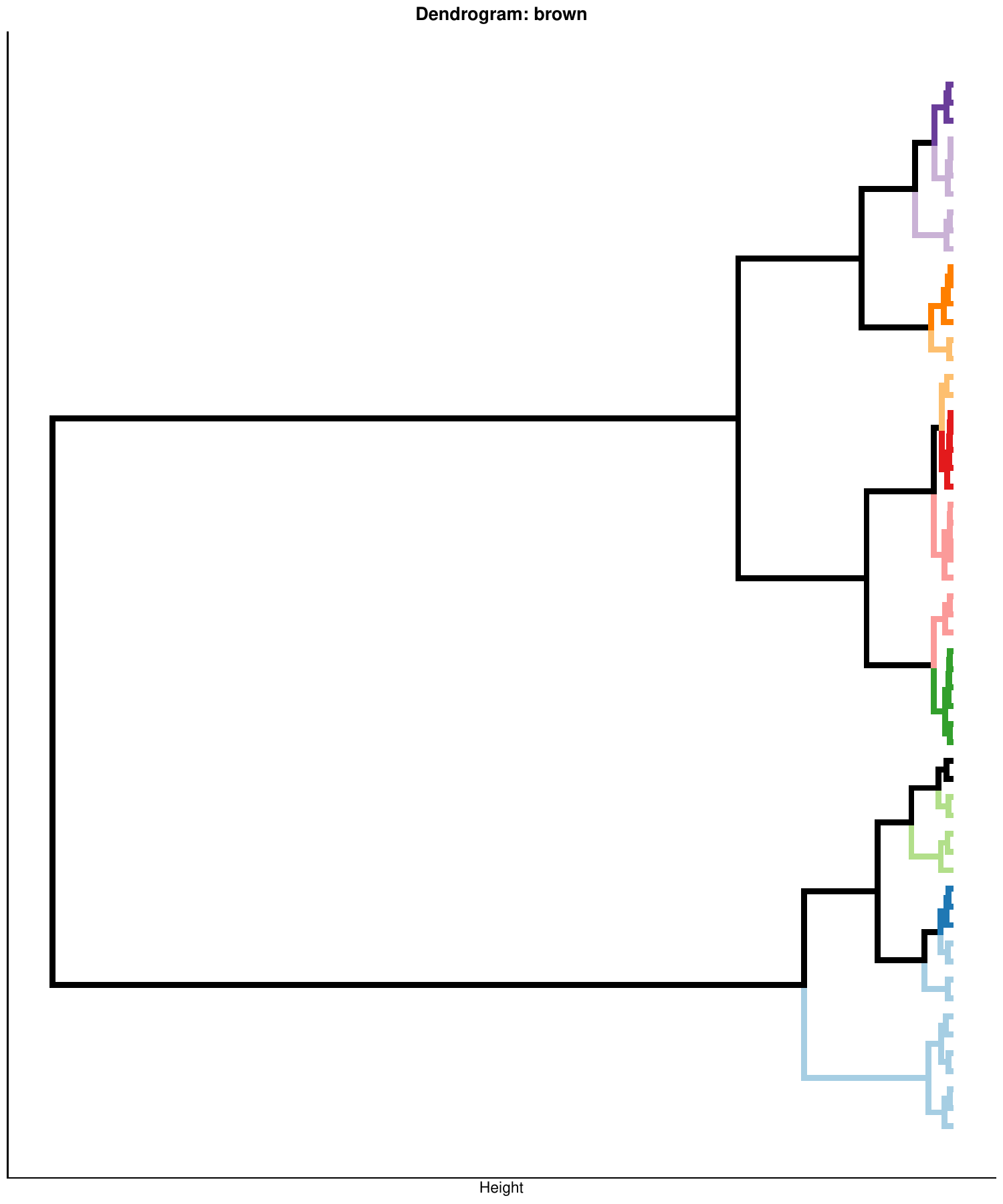
Results are also written to Results/Cell.groups.composition.csv and Results/Cell.groups.scores.csv. Passing dendrogram_file (and return_dendrogram = TRUE) additionally saves, per TF module, the dendrogram of correlated cell-type features that gets cut into cell groups:

Extract latent factors

Cell group scores are decomposed into NMF latent factors to obtain a compact, non-negative representation of the TME landscape. The rank argument controls the number of factors; if NULL, it is selected automatically.

latent_spaces <- compute.latent_factors(
  X         = cell_groups[[1]],
  rank      = NULL,
  seed      = 123,
  file_name = "Tutorial",
  return    = TRUE
)

The result is a list whose $Z element is a samples × factors matrix — the primary input for downstream statistical tests and machine learning.

# Access the factor scores matrix (samples x factors)
head(latent_spaces$Z)

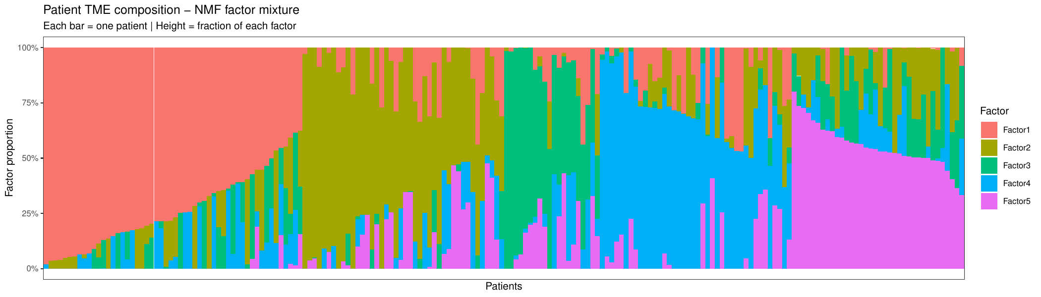
When return = TRUE, a stacked bar plot summarizing each patient’s mixture of latent factors is saved to Results/:

Extract cell niches

Cell niches are derived from latent factors by enriching each factor for specific cell-type signals from the deconvolution output. This step characterises each latent factor with a biological cell-type context.

cells_niches <- compute_cells_niches(
  latent_spaces   = latent_spaces,
  dt              = dt,
  cell.groups     = cell_groups,
  enrich_thresh   = 1.5,
  quantile_cutoff = 0.7,
  return          = TRUE,
  file_name       = "Tutorial"
)

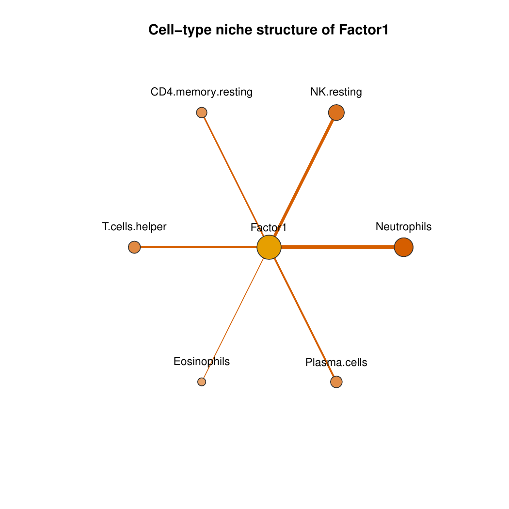
For each enriched latent factor, a star-network plot is saved showing which cell types define its niche (edge width reflects enrichment strength):

Next steps

With latent_spaces in hand, you can:

• Characterise TME states via GSEA and meta-program mapping → TME States
• Test clinical associations of latent factors → Statistical Analysis
• Train ML models on latent_spaces$Z → Machine Learning